Generative models, their latent spaces, geometry and identifiability

Latent spaces are central to many modern generative models, whether explicitly introduced through a bottleneck or implicitly defined by hidden states, as in VAEs, diffusion models, flows, and GANs.

In some models, such as diffusion models or GANs, the latent space may play a secondary role, with the main focus on sample quality and computational efficiency. However, when these models have real-world consequences, it becomes important to consider their reliability, interpretability, and explainability. In such cases, the latent space can serve as a useful tool.

In models like VAEs, the latent representation is more central and helps describe both the data-generating process and the structure behind the data. Researchers in fields such as biology, neuroscience, physics, chemistry, and the social sciences often rely on these representations to interpret complex data and make predictions [7,8].

A major challenge in both contexts is the lack of identifiability in the latent space. This refers to the fundamental impossibility of uniquely recovering the latent variables from observed data. This limitation, which has been formally established, affects the reliability of predictions and complicates efforts to learn representations that are interpretable, disentangled, or aligned with causal structure.

While the problem, as stated above, is fundamentally unsolvable, a substantial body of research has focused on characterizing it and proposing potential workarounds. Many of these approaches, however, rely either on additional data, which may be expensive or impractical to collect, or on restrictive modeling assumptions that constrain the model’s flexibility and expressiveness.

However, in many scientific and practical applications, what matters most is not the specific values of two latent variables, but the relationships between them. More broadly, interpretability often depends on comparisons made within a context. In practice, latent representations are frequently used in downstream tasks that rely on some notion of similarity, such as clustering, classification, or regression. This observation allows us to take a relational approach and reframe the problem through a geometric lens.

Viewed this way, the identifiability problem reduces to a simple postulate:

Geometric relations in the latent space should depend on the data, not on how we choose to represent it

This intuitive idea dates back to cartographers making maps of the Earth (representations in 2D latent space) and is a cornerstone of Einstein’s theory of general relativity, where the geometry of spacetime is independent of the coordinate system used to describe it.

Inspired by this concept, we show how identifiability in generative models can be reframed as a problem of the intrinsic geometry of data and its latent representation. This approach not only offers a principled way to address the problem but also provides fresh insights into the current state of the art in identifiability of generative models.

In what follows, we assume familiarity with generative models, particularly latent variable models. While some prior knowledge of differential geometry is helpful, we will introduce the necessary concepts informally and intuitively. For a rigorous treatment, we encourage readers to consult the full paper.

This post is organized as follows:

• Latent space geometry: How to equip the latent space with a meaningful geometry
• Identifiability: From identifiability of model parameters to maps between latent spaces of equivalent models
• Identifiable metric structures: Identifiable latent space geometry and what it reveals about the models we fit
• Take-aways: A concise summary of the key points to remember

Latent space geometry

Given high dimensional data representing observed phenomena such as images, audio, text, or protein sequences, we often assume the underlying mechanisms have lower intrinsic dimension. Therefore, learning useful representations of these high dimensional observations should be closely tied to uncovering the lower dimensional latent structure.

The central object for learning such representations in latent variable models is the generator (decoder) function, that is a smooth mapping:

that transforms latent variables $ \mathbf{z} \in \mathbb{R}^d $ into observed data $ \mathbf{x} \in \mathbb{R}^D $, assuming that $ d \leq D $. The decoder effectively discovers the data manifold embedded in the observed space and provides a way to transfer the geometry of this manifold back into the latent space.

To formalize this, we start with the notion of a manifold. In simple terms, a manifold is a space that looks Euclidean when examined locally. We can think of it as a surface that is flat in small neighborhoods but may have a more complex, curved global shape. The global structure emerges by smoothly joining these local neighborhoods.

Our decoder serves as a bridge between local neighborhoods in the latent space and their counterparts on the data manifold. Since the neighborhood around a point on the manifold is Euclidean, it naturally carries the standard inner product. We can then pull back this local geometry from the manifold to the latent space. This approach is established in differential geometry literature and is known as the pullback metric.

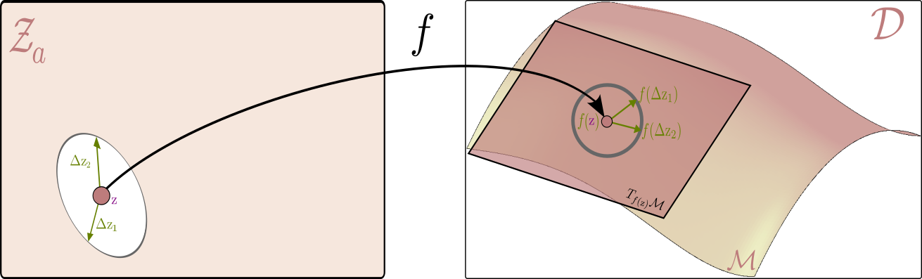
To recover this metric, consider a point $\textcolor{#800080}{\mathbf{z}}$ in the latent space and two small perturbations around it, $\textcolor{#017100}{\Delta \mathbf{z}_1}$, $\textcolor{#017100}{\Delta \mathbf{z}_2}$ around this point. In a local neighborhood of $\textcolor{#800080}{\mathbf{z}}$, we approximate the generator function using a first-order Taylor expansion:

where $\mathbf{J}_{\textcolor{#800080}{\mathbf{z}}}$ is the Jacobian of the generator function $f(\mathrm{z})$ with respect to the latent variables $ \mathrm{z} $.It is helpful to think of the Jacobian as a linear map that takes small changes in the latent space and translates them into changes in the data space.

Using this, we can now compute the distance between two perturbed points in the data space as follows:

where the pullback metric is given by the smooth function

that at each point $\mathbf{z}$ gives a symmetric positive definite matrix defining the inner product between two vectors $\textcolor{#017100}{\Delta \mathbf{z}_1}$ ,$\textcolor{#017100}{\Delta \mathbf{z}_2}$

This construction is not only an intuitive and practical way to define a metric, but it also has a key property needed for our geometric analysis.

To summarize, using a decoder and the pullback metric, we capture the geometric structure of the data manifold in terms of local coordianates (the latent space). Can we then be sure that this metric is meaningful and does not depend on the particular parametrization of the manifold?

In standard differential geometry, if two functions $f_a$ and $f_b$ both parameterize the same manifold, then their pullback metrics $\mathbf{g}_{a}$ and $\mathbf{g}_{b}$ are related by a smooth, one-to-one, map known as a diffeomorphism. Crucially, this transformation is an isometry, meaning it preserves the geometric structure of the data manifold. This means that once we define a pullback metric, it provides a well-defined and intrinsic description of the manifold’s geometry, independent of the specific parameterization.

The pullback metrics $\mathbf{g}_{a}$ and $\mathbf{g}_{b}$ are related by an isometry, meaning the geometry is preserved and does not depend on how the manifold is parameterized.

In terms of latent space geometry, this already sounds like we have what we want. Namely a meaningful metric that is invariant to the parametrization of the manifold.

However, we still need to connect this to the identifiability problem. Starting from the identifiability of model parameters, we need a way to analyze the problem in terms of a map between latent spaces of equivalent models - an indeterminacy transformation. If we can show that all indeterminacy transformations are isometries of their respective pullback metrics, then we can conclude that the general pullback metric is identifiable. This will be our strategy for the rest of the post.

An indeterminacy transformation is a map between latent spaces of equivalent models connecting the latent variables of one model to those of another and relating their marginal distributions.

Identifiability

In statistical literature, model parameters usually refer to the raw weights—the concatenated vector of values $\theta$ that define a specific instance of the model. For a latent variable model, two models with parameters $\theta_a$ and $\theta_b$ are considered equivalent if they define the same distribution over the data:

where

and the parameters $\theta$ are the concatenated weights of the generator function $f$ and the latent distribution $P(\mathrm{z})$. (In what follows, we will think of the latent codes $\mathrm{z}$ as realizations of a stochastic variable $Z$ living in a latent space $\mathcal{Z}$, and use $ P_{Z}$ as a short-hand notation for their marginal distribution.)

In plain language, the identifiability problem refers to situations where multiple distinct sets of parameters define the same distribution over observed data, making them indistinguishable in practice.

In the context of latent variable models, an alternative but equivalent perspective on model parameters was proposed by Johnny Xi and Ben Bloem-Reddy in their paper on Indeterminacy in Generative Models. They introduce a small abstraction: instead of focusing on raw weights, they define a model by the pair consisting of a generator function and its associated latent distribution. That is, \(\theta_a=(P_{Z_{a}}, f_a)\)

Thus, we no longer work in the space of weights, but rather in the space of pairs of distributions and generator functions.

Under this view, two models are equivalent if they produce the same distribution over observed data, even if their latent distributions and generator functions differ. This situation is illustrated in the figure below: two models generate the same data distribution, but differ in their latent structures and generator mappings.

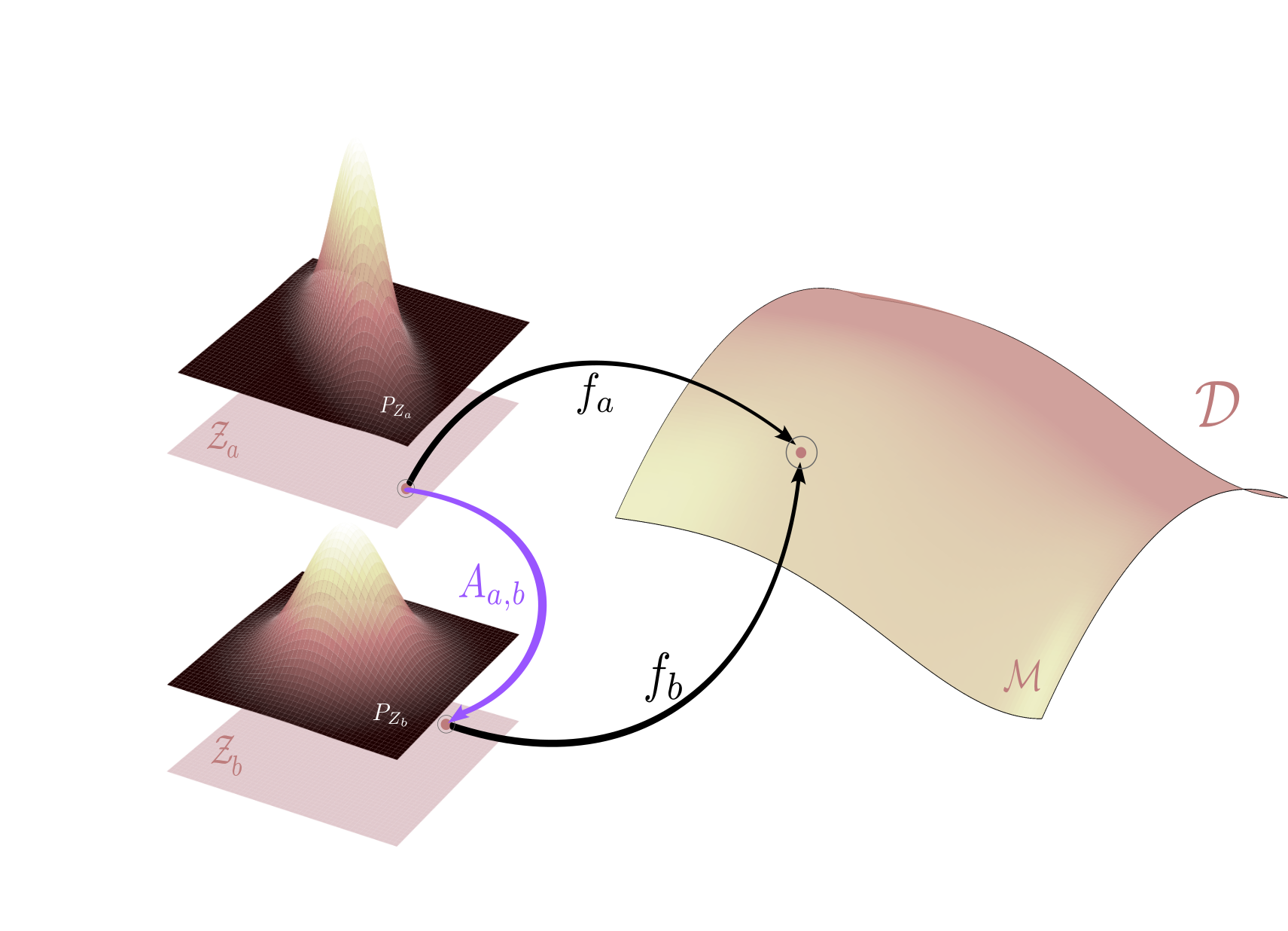
While this shift in perspective may seem abstract at first, it provides a powerful lens for analyzing the identifiability problem in latent variable models through transformations between latent spaces, denoted $ \textcolor{#9058F3}{A_{a,b}} $ as visualized above.

The paper by Xi & Bloem-Reddy shows that any valid indeterminacy transformation is probabilistically equivalent to moving back and forth along the generator functions. In other words, to move from one latent space $ \mathcal{Z}_a $ to another $ \mathcal{Z}_b $ we first map $ \mathcal{Z}_a $ to the data manifold by $f_a $, and then to the $ \mathcal{Z}_b $ through the inverse of $ f_b $. This leads to the following formulation:

All indeterminacy transformations between latent spaces of equivalent models are of the form $ \textcolor{#9058F3}{A_{a,b}}(\mathrm{z}) := f_b^{-1} \circ f_a(\mathrm{z}) $.

Now that we have a map $ \textcolor{#9058F3}{A_{a,b}}(\mathrm{z}) $ between latent spaces of equivalent models, we can analyze its properties. The goal is to establish that this transformation is a diffeomorphism and an isometry with respect to the pullback metric, which would imply that the pullback metric is identifiable.

Identifiable metric structures

From the previous section, we now know that for any two equivalent models $ \theta_a $ and $ \theta_b $, the transformation between their latent spaces is given by the indeterminacy transformation

More importantly, given a set of equivalent models, all possible indeterminacy transformations take this form.

Our treatment of $ \textcolor{#9058F3}{A_{a,b}}(\mathrm{z}) $ starts from its components: $ f_a $ and $ f_b^{-1} $. For this construction to be meaningful, We assume that the generator functions are one-to-one (injective) and map to the same image in the ambient space. Together with standard regularity conditions, this ensures that the image of $ f_a $ forms a smooth manifold in the ambient space. As a result, $ \textcolor{#9058F3}{A_{a,b}}(\mathrm{z}) $ becomes a smooth reparameterization, a diffeomorphism, of the same manifold.

Throughout, we refer to both the latent space and its image in the ambient space via $ f $ as manifolds. Although it may feel confusing, it is allowed since these objects are made equivalent (in geometric terms) by the decoder function.

Since equivalent latent spaces are related by $\textcolor{#9058F3}{A_{a,b}}$, the final step is to show that such transformations are isometries with respect to the pullback metric. This is the central result of our paper, where we demonstrate that $\textcolor{#9058F3}{A_{a,b}} $ satisfies the definition of an isometry.

The formal proof is given in the paper, but the intuition is simple and goes back to the section on latent space geometry: the decoders describe the same data manifold. Since the manifold itself is unchanged, its local neighborhoods must also be preserved under a diffeomorphism $\textcolor{#9058F3}{A_{a,b}}$, even if they are expressed in different coordinate systems. Thus, the pullback metrics $\mathbf{g}_{a}$ and $\mathbf{g}_{b}$ describe the same geometry and are related by an isometry $\textcolor{#9058F3}{A_{a,b}}$. Since all indeterminacy transformations are of this form, we conclude that the pullback metric is identifiable.

What can we reliably measure in the latent space?

The main result above guarantees that any geometric quantity defined through the pullback metric is identifiable. This means we can reliably compute distances, angles, and volumes in the latent space, and these measurements will remain consistent regardless of the specific generator function used.

The figure below illustrates this principle: it shows how to measure the length of a curve on the data manifold, and how the pullback metric allows us to perform this computation directly in the latent space.

Given the latent space on the left and ambient space on the right, the flat $ \mathcal{Z}_a $ serves as a map of the data manifold $ \mathcal{M} $ on the right. On the right, we can see a tangent plane to the manifold at each point $ f(\mathrm{z}) $ corresponding to the latent variable $ \mathrm{z} $. The picture is drawn in a way where the unit circle in the tangent plane corresponds to the unit ellipse in the latent space. All vectors within the circle (and the ellipsis) are of unit length, but whereas the ones on the right are Euclidean, the ones on the left are measured with respect to the pullback metric.

Using this intuition, we can now, for example, measure the distance between two points on the data manifold $ (\mathrm{z}_1,\mathrm{z}_2) $ by finding a shortest path (geodesic) between them. In practice, this is done by optimizing the energy of a curve $ \eta $ in the latent space that corresponds to the path $\gamma$ on the data manifold ($\gamma(t)=f\circ \eta(t)$). I.e. the following optimization problem:

where $ ||\dot{\eta}(t)||_{\mathbf{g}}^2 = \dot{\eta}(t)^\top \mathbf{g}(\eta(t)) \dot{\eta}(t) $ is the pullback metric at the point $ \eta(t) $ and eta is a curve in the latent space that starts at $ \eta(0) = \mathrm{z}_1 $ and ends at $ \eta(1) = \mathrm{z}_2 $.

The result of this optimization is guaranteed to be identifiable: it will yield the same distance even when using another equivalent model with a differently shaped latent space.

Does it work in practice?

The short answer is yes. The longer answer depends on how we define success in practice.

The form of the indeterminacy transformations $ \textcolor{#9058F3}{A_{a,b}}(\mathrm{z}) $ from the section on identifiability is proven in the limit of infinite data. While such theoretical limits are common in statistics, real-world models are trained on finite data, meaning they do not learn the true data manifold exactly and their approximations are inherently noisy. In addition, both the identifiability theory and our geometric construction assume that the generator functions are injective. This assumption is milder than what is typically required for identifiability, but still a constraint we would prefer to relax in practice.

These two considerations mean that, although the theory provides strong guarantees, we should expect some variability in the measurements performed in the latent space using the pullback metric. The good news is that this variability is consistently lower than that of measurements made using the standard Euclidean metric. Moreover, relaxing the injectivity assumption does not appear to negatively affect practical performance.

Experiment setup: to illustrate this, we compute the coefficient of variation of the distances (geodesic and Euclidean) between same pairs of points in the latent space across 30 model retrainings.

1.train 30 models on the training set using different random seeds
2.randomly sample 100 pairs in the test set
    for each point pair:
        for each model:
            1.encode the sampled pairs into the latent space
            2.compute the distance between the pairs using the pullback metric and the Euclidean metric
        return the distances for each model
        for each metric:
            compute the coefficient of variation of the distances across all models
      return the coefficient of variation for each distance metric
return the vector of coefficient of variation for each distance metric between each pair of points

A successful experiment should yield a lower coefficient of variation for the geodesic distnaces compared to the Euclidean metric. We visualize the results using histograms of the coefficient of variation for each dataset and each metric. For code and detais, see the GitHub repository.

Our injective decoder is based on the $ \mathcal{M} $-flow architecture [3] and applied to the MNIST and CIFAR10 datasets.

A geodesic parametrized by a spline in the 2D latent space of the $ \mathcal{M} $-flow model trained on 3 digit subset of MNIST.

In the figure below, we show the histograms of the coefficient of variation and observe that the geodesic distance has a lower coefficient of variation than the Euclidean distance measure.

(Left): Histogram for the MNIST dataset. (Right): Histogram for the CIFAR10.

Relaxing the injectivity constraint as we train a CNN based VAE on FMNIST and CelebA datasets. Below we show the histograms of the coefficient of variation and observe that the geodesic distance metric consistently has a lower and narrower coefficient of variation than the Euclidean metric.

(Left): Histogram for the FMNIST dataset. (Right): Histogram for the CelebA.

The overlapping histograms above need a comment: apart from stochastics and approximations inducing noise into fitting a data manifold and calculating the geodesic distances on it, there are reasons within our geometric framework that can lead to overlapping histograms. As alluded to in the section above, when the data manifold is flat, the Euclidean metric can be identifiable and we do not gain an extra benefit from using the pullback metric. Furthermore, when the data manifold is not flat, there can still be areas where the Euclidean metric is a good proxy for the pullback metric. This is especially true when the points are very close to each other.

To see what these high-dimensional curves look like in practice we show an interpolation between two points in the latent space of a VAE trained on CelebA dataset. While both seem to follow the data manifold without major differences, we see that the geodesic curve satisfies the constant speed traversal property by observing the appearence of glasses earlier.

Interpolation according to the geodesic (top) and the Euclidean (bottom) curves in the latent space

What if we really want the Euclidean metric in the latent space to be identifiable?

In this section, we apply what we know about identifiability through $ \textcolor{#9058F3}{A_{a,b}}(\mathrm{z}) $ in the context of contemporary literature. Ideas such as iVAE [6] and identifiability through multiple views [4,5] are based on the assumption that the latent space is Euclidean, and implicitly, they aim to make the Euclidean metric identifiable. Apart from imposing restrictions on the model or requiring additional labeled data, we show that the success of these approaches relies on another implicit assumption: the data manifold is flat, i.e., it can be represented as a Euclidean space.

Euclidean metric can only be identifiable if the data manifold is flat

This is easy to see since we established identifiability of the pullback metric by showing that $ \textcolor{#9058F3}{A_{a,b}}(\mathrm{z}) $ is an isometry. Assuming that our pullack metric is Euclidean, then it is identifiable if all $ \textcolor{#9058F3}{A_{a,b}}(\mathrm{z}) $ are isometries of Euclidean space. By definition, this is only possible if the data manifold is flat, i.e. the metric $\mathbf{g}(\mathrm{z})$ does not depend on the point $\mathrm{z}$, and is constant across the latent space.

Quick notes

• We have assumed the Euclidean metric in the ambient space to calculate the dot product. However, this is not a limitation as the pullback metric can be defined for any valid ambient metric.

• There are many ways to calculate (approximate) the geodesic distance in the latent space. We choose to parametrize the geodesic by a spline and optimize the energy of the curve using gradient descent. For details, see the appendix of the paper and the code repository.

• Computing geometric relations using pullback geometry undeniably comes with extra computational burden. We argue, however, that it is manageble and many efficient methods exist [2,9].

Take-aways

• Latent spaces play a central role in scientific uses of generative and deep latent variable models. When identifiable, they can support interpretability, explainability, and reliability in applications with real-world impact.

• Identifiability of latent representations is provably impossible, which motivates our shift toward a relational perspective.

• Geometric relations between latent variables can be identified when the geometry of the data manifold is taken into account.

• Ignoring the geometry of the data manifold amounts to assuming it is flat.

• Our approach is scalable, entirely post-hoc, and does not require labeled data or restrictive modeling assumptions.

Ackgnowledgements

Big thanks for feedback to Yevgen Zainchkovskyy, Samuel Matthiesen and Federico Bergamin. The diagrams were either made or influenced by Søren Hauberg.

References:

[1] Xi, Q. & Bloem-Reddy, B.. (2023). Indeterminacy in Generative Models: Characterization and Strong Identifiability. Proceedings of The 26th International Conference on Artificial Intelligence and Statistics, in Proceedings of Machine Learning Research 206:6912-6939 Available from https://proceedings.mlr.press/v206/xi23a.html.

[2] Syrota, S., Moreno-Muñoz, P. & Hauberg, S.. (2024). Decoder ensembling for learned latent geometries. Proceedings of the Geometry-grounded Representation Learning and Generative Modeling Workshop (GRaM), in Proceedings of Machine Learning Research 251:277-285 Available from https://proceedings.mlr.press/v251/syrota24a.html.

[3] Brehmer, J., & Cranmer, K. (2020). Flows for simultaneous manifold learning and density estimation. Advances in neural information processing systems, 33, 442-453.

[4]Gresele, L., Rubenstein, P. K., Mehrjou, A., Locatello, F., & Schölkopf, B. (2020, August). The incomplete rosetta stone problem: Identifiability results for multi-view nonlinear ica. In Uncertainty in Artificial Intelligence (pp. 217-227). PMLR.

[5] Locatello, F., Poole, B., Rätsch, G., Schölkopf, B., Bachem, O., & Tschannen, M. (2020, November). Weakly-supervised disentanglement without compromises. In International conference on machine learning (pp. 6348-6359). PMLR.

[6] Khemakhem, I., Kingma, D., Monti, R., & Hyvarinen, A. (2020, June). Variational autoencoders and nonlinear ica: A unifying framework. In International conference on artificial intelligence and statistics (pp. 2207-2217). PMLR.

[7] Schneider, S., Lee, J.H. & Mathis, M.W. Learnable latent embeddings for joint behavioural and neural analysis. Nature 617, 360–368 (2023). https://doi.org/10.1038/s41586-023-06031-6

[8] Detlefsen, N.S., Hauberg, S. & Boomsma, W. Learning meaningful representations of protein sequences. Nat Commun 13, 1914 (2022). https://doi.org/10.1038/s41467-022-29443-w

[9] Rygaard, F. M., & Hauberg, S. (2025). GEORCE: A Fast New Control Algorithm for Computing Geodesics. arXiv preprint arXiv:2505.05961.